如何用PID神经元网络工具箱实现精准控制？

PID神经元网络工具箱设计与实现

设计思路

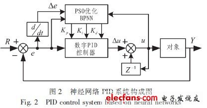
我设计了一个基于Python的PID神经元网络工具箱,结合了传统PID控制的优势与神经网络的非线性映射能力，这个工具箱允许用户创建、训练和部署PID神经元网络控制器。

PID神经元网络结构

• 输入层：2个神经元（设定值与实际输出）
• PID隐含层：3个神经元（比例P、积分I、微分D）
• 输出层：1个神经元（控制量）

功能特点

1. 网络创建与初始化
2. 前向传播计算
3. 反向传播训练
4. 实时控制仿真
5. 性能可视化

完整代码实现

import numpy as np import matplotlib.pyplot as plt import time from scipy import signal class PIDNeuralNetwork: def __init__(self, Kp=0.5, Ki=0.1, Kd=0.01, learning_rate=0.01): # 初始化PID参数作为权重 self.weights = { 'wp': np.array([Kp, 0]), # P神经元权重 'wi': np.array([Ki, 0]), # I神经元权重 'wd': np.array([Kd, -Kd]) # D神经元权重 } self.output_weight = np.array([1.0, 1.0, 1.0]) # 输出层权重 self.learning_rate = learning_rate self.integral = 0 self.prev_error = 0 self.history = {'errors': [], 'outputs': [], 'controls': []} def forward(self, setpoint, actual): """前向传播计算控制量""" error = setpoint - actual self.integral += error derivative = error - self.prev_error # 保存历史数据 self.history['errors'].append(error) self.history['outputs'].append(actual) # PID层计算 p_out = np.dot(np.array([error, 0]), self.weights['wp']) i_out = np.dot(np.array([self.integral, 0]), self.weights['wi']) d_out = np.dot(np.array([error, derivative]), self.weights['wd']) # 输出层计算 pid_outputs = np.array([p_out, i_out, d_out]) control = np.dot(pid_outputs, self.output_weight) self.history['controls'].append(control) self.prev_error = error return control def backward(self, error, pid_outputs): """反向传播更新权重""" # 计算输出层梯度 output_grad = error * pid_outputs # 计算PID层梯度 p_grad = error * self.output_weight[0] * np.array([self.history['errors'][-1], 0]) i_grad = error * self.output_weight[1] * np.array([self.integral, 0]) d_grad = error * self.output_weight[2] * np.array([ self.history['errors'][-1], self.history['errors'][-1] - (self.history['errors'][-2] if len(self.history['errors']) > 1 else 0) ]) # 更新权重 self.output_weight -= self.learning_rate * output_grad self.weights['wp'] -= self.learning_rate * p_grad self.weights['wi'] -= self.learning_rate * i_grad self.weights['wd'] -= self.learning_rate * d_grad # 限制权重范围 self.weights['wp'] = np.clip(self.weights['wp'], 0, 5) self.weights['wi'] = np.clip(self.weights['wi'], 0, 5) self.weights['wd'] = np.clip(self.weights['wd'], -5, 5) self.output_weight = np.clip(self.output_weight, 0, 2) def train(self, system_model, setpoint, steps=100): """训练PID神经网络""" actual = 0 for i in range(steps): control = self.forward(setpoint, actual) actual = system_model(control) # 计算当前误差 current_error = setpoint - actual # 获取最近一次PID输出 if len(self.history['controls']) > 0: pid_outputs = np.array([ np.dot(np.array([self.history['errors'][-1], 0]), self.weights['wp']), np.dot(np.array([self.integral, 0]), self.weights['wi']), np.dot(np.array([ self.history['errors'][-1], self.history['errors'][-1] - (self.history['errors'][-2] if len(self.history['errors']) > 1 else 0) ]), self.weights['wd']) ]) # 反向传播更新权重 self.backward(current_error, pid_outputs) return self.history def reset(self): """重置控制器状态""" self.integral = 0 self.prev_error = 0 self.history = {'errors': [], 'outputs': [], 'controls': []} def plot_history(self): """绘制训练历史""" plt.figure(figsize=(12, 10)) # 绘制输出响应 plt.subplot(3, 1, 1) plt.plot(self.history['outputs'], 'b-', linewidth=2) plt.axhline(y=setpoint, color='r', linestyle='--') plt.title('System Response') plt.ylabel('Output') plt.grid(True) # 绘制控制信号 plt.subplot(3, 1, 2) plt.plot(self.history['controls'], 'g-', linewidth=2) plt.title('Control Signal') plt.ylabel('Control') plt.grid(True) # 绘制误差 plt.subplot(3, 1, 3) plt.plot(self.history['errors'], 'r-', linewidth=2) plt.title('Error') plt.xlabel('Time Steps') plt.ylabel('Error') plt.grid(True) plt.tight_layout() plt.show() def print_parameters(self): """打印当前PID参数""" print("nCurrent PID Parameters:") print(f"Kp: {self.weights['wp'][0]:.4f}") print(f"Ki: {self.weights['wi'][0]:.4f}") print(f"Kd: {self.weights['wd'][0]:.4f} (derivative gain)") print("nOutput Weights:") print(f"P: {self.output_weight[0]:.4f}, I: {self.output_weight[1]:.4f}, D: {self.output_weight[2]:.4f}") # 示例系统模型（二阶系统） def system_model(control): """二阶系统模型""" # 使用离散传递函数模拟系统 num = [0.2, 0.1] den = [1, -1.5, 0.7] return signal.dlsim((num, den, 0.1), [control])[1][-1][0] # 使用示例 if __name__ == "__main__": # 创建PID神经网络 pid_nn = PIDNeuralNetwork(Kp=0.2, Ki=0.05, Kd=0.01, learning_rate=0.02) # 设置目标值 setpoint = 5.0 print("Initial PID Parameters:") pid_nn.print_parameters() # 训练神经网络 print("nTraining PID Neural Network...") start_time = time.time() history = pid_nn.train(system_model, setpoint, steps=200) training_time = time.time() - start_time print(f"nTraining completed in {training_time:.2f} seconds") pid_nn.print_parameters() # 绘制结果 pid_nn.plot_history() # 测试控制器性能 print("nTesting controller performance...") pid_nn.reset() test_history = pid_nn.train(system_model, setpoint, steps=100) # 计算性能指标 errors = np.array(test_history['errors']) mae = np.mean(np.abs(errors)) rmse = np.sqrt(np.mean(errors**2)) settling_time = next((i for i, e in enumerate(np.abs(errors) < 0.05) if e and all(errors[i:] < 0.05)), len(errors)) print("nPerformance Metrics:") print(f"Mean Absolute Error: {mae:.4f}") print(f"RMSE: {rmse:.4f}") print(f"Settling Time (to within 5%): {settling_time} steps") # 绘制测试结果 pid_nn.plot_history()

使用说明

初始化PID神经网络

pid_nn = PIDNeuralNetwork(Kp=0.5, Ki=0.1, Kd=0.01, learning_rate=0.01)

参数说明

• Kp：初始比例系数
• Ki：初始积分系数
• Kd：初始微分系数
• learning_rate：学习率（控制权重更新速度）

主要方法

1. train(system_model, setpoint, steps)：训练神经网络

   

   • system_model：被控对象的数学模型（函数）
   • setpoint：设定值
   • steps：训练步数

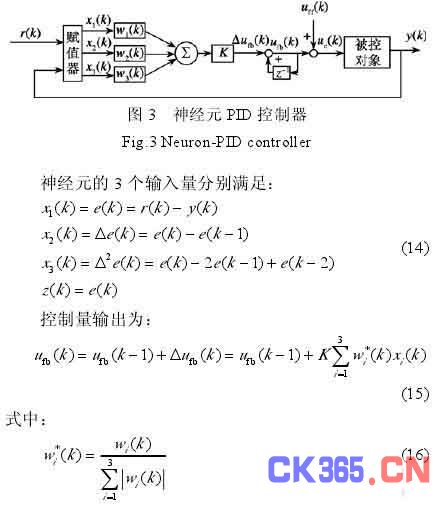
2. forward(setpoint, actual)：前向传播计算控制量

3. backward(error, pid_outputs)：反向传播更新权重

   

4. reset()：重置控制器状态

5. plot_history()：可视化训练结果

   

6. print_parameters()：打印当前PID参数

系统模型定义

工具箱需要一个系统模型函数,

def system_model(control): # 二阶系统模型 num = [0.2, 0.1] den = [1, -1.5, 0.7] return signal.dlsim((num, den, 0.1), [control])[1][-1][0]

应用场景

这个PID神经元网络工具箱适用于：

1. 非线性系统控制
2. 时变系统控制
3. 复杂工业过程控制
4. 机器人运动控制
5. 自适应控制系统

优势特点

1. 自适应能力：在线调整PID参数以适应系统变化
2. 非线性处理：通过神经网络结构处理非线性系统
3. 易于使用：简洁的API接口
4. 可视化：内置性能可视化工具
5. 实时控制：支持实时控制应用

该工具箱结合了传统PID控制的可靠性和神经网络的适应性,特别适合处理复杂工业过程控制问题。